Data curation
Initial instructions:
This tutorial was designed to demonstrate how to use the ULaMDyn package as a python API for collecting data from the outputs of NAMD trajectories generated by the Newton-X program. The ULaMDyn API provides a flexible framework to manipulate the information collected by the program and structured into pandas DataFrame objects either via interactive Jupyter environment or by developing customized scripts for specific purposes.
You should be inside of the TRAJECTORIES directory in your Newton-X calculation.
Ulamdyn will look for the file control.dyn, which should be inside of TRAJECTORIES.
Import the modules you are going to use.
[1]:
import ulamdyn as umd
import pandas as pd
import numpy as np
GetProperties:
Read and process all properties available in the outputs of Newton-X MD trajectories (RESULTS directory). In this class, there are several methods implemented to extract specific information: energies(), oscillator_strength(), populations() and save_csv.
Energy quantities processed by this class are transformed from u.a. to eV. For the other properties, the original units used in NX are kept.
[2]:
# Instanciate the class:
properties = umd.GetProperties()
1. energies():
Read and process the energy information from the en.dat (classical NX) or .h5 (new NX) file and return a processed pandas dataframe with the information of all trajectories stacked.
[3]:
df_en = properties.energies()
df_en.head()
Reading energies from TRAJ1...
Reading energies from TRAJ2...
Reading energies from TRAJ3...
Reading energies from TRAJ4...
Reading energies from TRAJ5...

-----------------------------------------------------
The properties dataset is empty.
Updating class variable with the current loaded data.
-----------------------------------------------------
[3]:
| TRAJ | time | State | Total_Energy | Hops_S12 | S1 | Hops_S21 | DE21 | |
|---|---|---|---|---|---|---|---|---|
| 0 | 1 | 0.0 | 2 | -6271.713990 | 0 | -6276.740507 | 0 | 3.852182 |
| 1 | 1 | 0.1 | 2 | -6271.714018 | 0 | -6276.777841 | 0 | 3.839637 |
| 2 | 1 | 0.2 | 2 | -6271.714045 | 0 | -6276.812753 | 0 | 3.825025 |
| 3 | 1 | 0.3 | 2 | -6271.714072 | 0 | -6276.844754 | 0 | 3.808371 |
| 4 | 1 | 0.4 | 2 | -6271.714099 | 0 | -6276.873408 | 0 | 3.789650 |
This dataframe shows the line number, the identifier of NX trajectory (TRAJ), the current state of the trajectory (State), the total energy, the hopings between the states (Hops_S12 and Hops_S21), the energy difference between the accessible states (DE21) and the absolute energy of the ground state.
[4]:
df_en.columns
[4]:
Index(['TRAJ', 'time', 'State', 'Total_Energy', 'Hops_S12', 'S1', 'Hops_S21',
       'DE21'],
      dtype='object')
Using the pandas functions, one can easily obtain a full description of the dataset generated by ulamdyn.
[5]:
df_en.describe()
[5]:
| TRAJ | time | State | Total_Energy | Hops_S12 | S1 | Hops_S21 | DE21 | |
|---|---|---|---|---|---|---|---|---|
| count | 2984.000000 | 2984.000000 | 2984.000000 | 2984.000000 | 2984.000000 | 2984.000000 | 2984.000000 | 2984.000000 |
| mean | 3.000000 | 29.795912 | 1.222185 | -6271.688662 | 0.000670 | -6274.989408 | 0.002346 | 3.280622 |
| std | 1.419419 | 17.241088 | 0.415785 | 0.150424 | 0.025885 | 0.935564 | 0.048385 | 1.823839 |
| min | 1.000000 | 0.000000 | 1.000000 | -6271.831571 | 0.000000 | -6277.687709 | 0.000000 | 0.020926 |
| 25% | 2.000000 | 14.900000 | 1.000000 | -6271.820060 | 0.000000 | -6275.582451 | 0.000000 | 1.769013 |
| 50% | 3.000000 | 29.800000 | 1.000000 | -6271.714317 | 0.000000 | -6274.911697 | 0.000000 | 3.242157 |
| 75% | 4.000000 | 44.700000 | 1.000000 | -6271.675133 | 0.000000 | -6274.352965 | 0.000000 | 4.641496 |
| max | 5.000000 | 60.000000 | 2.000000 | -6271.412352 | 1.000000 | -6272.713601 | 1.000000 | 7.197878 |
Counting the number of entries.
From this initial dataframe, it is already possible to capture some characteristics of the dataframe. For example, with count it is possible to check how many entries we have in the dataframe and with nunique we can obtain the number of unique values, that applied to the trajectories column, return the number of trajectories available in the directory.
[6]:
df_en.count()
[6]:
TRAJ            2984
time            2984
State           2984
Total_Energy    2984
Hops_S12        2984
S1              2984
Hops_S21        2984
DE21            2984
dtype: int64
[7]:
df_en['TRAJ'].nunique()
[7]:
5
Getting features of MD trajectories.
It is also possible to group the information available in the dataframe in a more convenient way. For example, by using the groupby function of pandas one can easily obtain the maximum time of the dynamics for each one of the trajectories read by the program.
[8]:
df_en.groupby(['TRAJ']).max()
[8]:
| time | State | Total_Energy | Hops_S12 | S1 | Hops_S21 | DE21 | |
|---|---|---|---|---|---|---|---|
| TRAJ | |||||||
| 1 | 60.0 | 2 | -6271.713854 | 0 | -6273.107350 | 1 | 6.510790 |
| 2 | 60.0 | 2 | -6271.674398 | 0 | -6273.463466 | 1 | 6.695882 |
| 3 | 57.9 | 2 | -6271.809829 | 1 | -6273.447465 | 1 | 6.806442 |
| 4 | 60.0 | 2 | -6271.828714 | 1 | -6273.092656 | 1 | 6.676670 |
| 5 | 60.0 | 2 | -6271.412352 | 0 | -6272.713601 | 1 | 7.197878 |
Selecting properties of hopping points
The command shown below is an example of how to filter the energy dataframe dataframe to display only the rows in which there is a hopping between states 1 and 2.
[9]:
hoppings_S12 = df_en[df_en['Hops_S12'] == 1 ]
hoppings_S12
[9]:
| TRAJ | time | State | Total_Energy | Hops_S12 | S1 | Hops_S21 | DE21 | |
|---|---|---|---|---|---|---|---|---|
| 1281 | 3 | 7.9 | 1 | -6271.823435 | 1 | -6274.287182 | 0 | 0.028545 |
| 1921 | 4 | 13.9 | 1 | -6271.830863 | 1 | -6274.562262 | 0 | 1.091885 |
From the filtered dataset shown above, one can easily identify relevant information related to the hopping time such as the energy gap between S0 and S1, given by the column “DE21”.
Visualizing time evolution of the potential energy
Energy of state 1:
To obtain the absolute value of root 2, i. e. S1 state, we need to add the DE21 gap (in eV) to the root1 potential energy (in atomic unities), i. e. S0. And then, add it to the dataframe as column.
[10]:
df_en['Root2'] = df_en['Total_Energy'] + df_en['DE21']
df_en
[10]:
| TRAJ | time | State | Total_Energy | Hops_S12 | S1 | Hops_S21 | DE21 | Root2 | |
|---|---|---|---|---|---|---|---|---|---|
| 0 | 1 | 0.0 | 2 | -6271.713990 | 0 | -6276.740507 | 0 | 3.852182 | -6267.861809 |
| 1 | 1 | 0.1 | 2 | -6271.714018 | 0 | -6276.777841 | 0 | 3.839637 | -6267.874380 |
| 2 | 1 | 0.2 | 2 | -6271.714045 | 0 | -6276.812753 | 0 | 3.825025 | -6267.889020 |
| 3 | 1 | 0.3 | 2 | -6271.714072 | 0 | -6276.844754 | 0 | 3.808371 | -6267.905701 |
| 4 | 1 | 0.4 | 2 | -6271.714099 | 0 | -6276.873408 | 0 | 3.789650 | -6267.924449 |
| ... | ... | ... | ... | ... | ... | ... | ... | ... | ... |
| 2979 | 5 | 59.6 | 1 | -6271.412760 | 0 | -6274.238936 | 0 | 5.447232 | -6265.965528 |
| 2980 | 5 | 59.7 | 1 | -6271.412760 | 0 | -6274.225956 | 0 | 5.497873 | -6265.914888 |
| 2981 | 5 | 59.8 | 1 | -6271.412760 | 0 | -6274.214527 | 0 | 5.548187 | -6265.864574 |
| 2982 | 5 | 59.9 | 1 | -6271.412733 | 0 | -6274.204813 | 0 | 5.598147 | -6265.814586 |
| 2983 | 5 | 60.0 | 1 | -6271.412733 | 0 | -6274.196922 | 0 | 5.647644 | -6265.765089 |
2984 rows × 9 columns
We can then later obtain filter the dataframe to obtain root 2 energy from a specific trajectory and use it to plot the potential energy surfaces of the relevant states.
Energy of the current state:
[11]:
df_en['only_root2'] = df_en[df_en['State'] == 2]['Root2']
df_en['only_root1'] = df_en[df_en['State'] == 1]['S1']
df_en = df_en.fillna(0.0)
df_en['Current'] = df_en['only_root2'] + df_en['only_root1']
df_en = df_en.drop(columns='only_root2').drop(columns='only_root1')
df_en
[11]:
| TRAJ | time | State | Total_Energy | Hops_S12 | S1 | Hops_S21 | DE21 | Root2 | Current | |
|---|---|---|---|---|---|---|---|---|---|---|
| 0 | 1 | 0.0 | 2 | -6271.713990 | 0 | -6276.740507 | 0 | 3.852182 | -6267.861809 | -6267.861809 |
| 1 | 1 | 0.1 | 2 | -6271.714018 | 0 | -6276.777841 | 0 | 3.839637 | -6267.874380 | -6267.874380 |
| 2 | 1 | 0.2 | 2 | -6271.714045 | 0 | -6276.812753 | 0 | 3.825025 | -6267.889020 | -6267.889020 |
| 3 | 1 | 0.3 | 2 | -6271.714072 | 0 | -6276.844754 | 0 | 3.808371 | -6267.905701 | -6267.905701 |
| 4 | 1 | 0.4 | 2 | -6271.714099 | 0 | -6276.873408 | 0 | 3.789650 | -6267.924449 | -6267.924449 |
| ... | ... | ... | ... | ... | ... | ... | ... | ... | ... | ... |
| 2979 | 5 | 59.6 | 1 | -6271.412760 | 0 | -6274.238936 | 0 | 5.447232 | -6265.965528 | -6274.238936 |
| 2980 | 5 | 59.7 | 1 | -6271.412760 | 0 | -6274.225956 | 0 | 5.497873 | -6265.914888 | -6274.225956 |
| 2981 | 5 | 59.8 | 1 | -6271.412760 | 0 | -6274.214527 | 0 | 5.548187 | -6265.864574 | -6274.214527 |
| 2982 | 5 | 59.9 | 1 | -6271.412733 | 0 | -6274.204813 | 0 | 5.598147 | -6265.814586 | -6274.204813 |
| 2983 | 5 | 60.0 | 1 | -6271.412733 | 0 | -6274.196922 | 0 | 5.647644 | -6265.765089 | -6274.196922 |
2984 rows × 10 columns
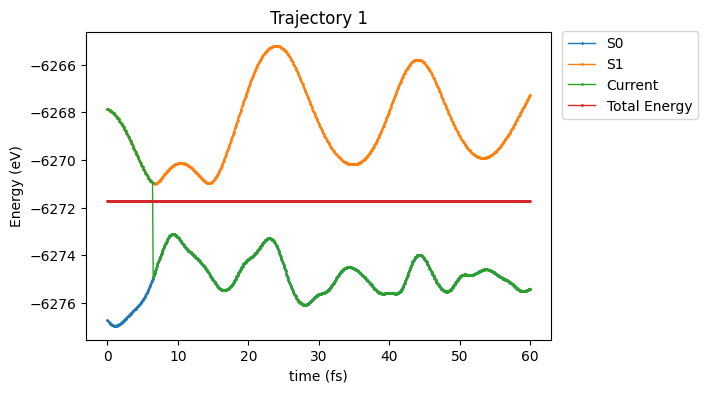
Plotting the results
[12]:
# First some code lines to set up the plot.
import matplotlib.pyplot as plt
fig , ax = plt.subplots(figsize=(6,4))

## 1. Subplot 1: Mean Population
# syntax: plt.subplot(number_lines, number_columns, selected_plot)
plt.subplot(1, 1, 1)

TRAJ_ID = 1

# syntax: plt.plot(x-axis, y-axis, series_label, type_marker, ...)
plt.plot(df_en[df_en['TRAJ'] == TRAJ_ID ]['time'], df_en[df_en['TRAJ'] == TRAJ_ID ]['S1'],           label='S0',           marker='o', linewidth=1, markersize=1)
plt.plot(df_en[df_en['TRAJ'] == TRAJ_ID ]['time'], df_en[df_en['TRAJ'] == TRAJ_ID ]['Root2'],        label='S1',           marker='o', linewidth=1, markersize=1)
plt.plot(df_en[df_en['TRAJ'] == TRAJ_ID ]['time'], df_en[df_en['TRAJ'] == TRAJ_ID ]['Current'],      label='Current',      marker='o', linewidth=1, markersize=1)
plt.plot(df_en[df_en['TRAJ'] == TRAJ_ID ]['time'], df_en[df_en['TRAJ'] == TRAJ_ID ]['Total_Energy'], label='Total Energy', marker='o', linewidth=1, markersize=1)

# x- and y-axis labels
plt.ylabel('Energy (eV)', fontsize=10)
plt.xlabel('time (fs)'  , fontsize=10)

# # Legend placement and style
plt.legend(loc='center right', bbox_to_anchor=(1.33, 0.86), frameon=None, ncol=1)
plt.title("Trajectory "+str(TRAJ_ID))
plt.show()
2. oscillator_strength():
This is a method of the GetProperties class that can be used to collect the oscillator strength computed by an external QM program during the dynamics simulation. After calling this method, the oscillator strength data collected from all trajectories will be merged with the existing properties dataset.
Note: The availability of the oscillator strength data depends on the QM program / method used to compute the electronic structure of the system. If available, ULaMDyn will collect this information from the RESULTS/properties file (classical NX) or from the .h5 file (new NX) for each MD trajectory.
[13]:
properties.oscillator_strength()
Reading oscillator strength from TRAJ1...
Reading oscillator strength from TRAJ2...
Reading oscillator strength from TRAJ3...
Reading oscillator strength from TRAJ4...
Reading oscillator strength from TRAJ5...
[13]:
| TRAJ | time | State | Total_Energy | Hops_S12 | S1 | Hops_S21 | DE21 | Root2 | only_root2 | only_root1 | f_21 | |
|---|---|---|---|---|---|---|---|---|---|---|---|---|
| 0 | 1 | 0.0 | 2 | -6271.713990 | 0 | -6276.740507 | 0 | 3.852182 | -6267.861809 | -6267.861809 | NaN | -0.004430 |
| 1 | 1 | 0.1 | 2 | -6271.714018 | 0 | -6276.777841 | 0 | 3.839637 | -6267.874380 | -6267.874380 | NaN | -0.004396 |
| 2 | 1 | 0.2 | 2 | -6271.714045 | 0 | -6276.812753 | 0 | 3.825025 | -6267.889020 | -6267.889020 | NaN | -0.004357 |
| 3 | 1 | 0.3 | 2 | -6271.714072 | 0 | -6276.844754 | 0 | 3.808371 | -6267.905701 | -6267.905701 | NaN | -0.004313 |
| 4 | 1 | 0.4 | 2 | -6271.714099 | 0 | -6276.873408 | 0 | 3.789650 | -6267.924449 | -6267.924449 | NaN | -0.004266 |
| ... | ... | ... | ... | ... | ... | ... | ... | ... | ... | ... | ... | ... |
| 2979 | 5 | 59.6 | 1 | -6271.412760 | 0 | -6274.238936 | 0 | 5.447232 | -6265.965528 | NaN | -6274.238936 | -0.006061 |
| 2980 | 5 | 59.7 | 1 | -6271.412760 | 0 | -6274.225956 | 0 | 5.497873 | -6265.914888 | NaN | -6274.225956 | -0.006146 |
| 2981 | 5 | 59.8 | 1 | -6271.412760 | 0 | -6274.214527 | 0 | 5.548187 | -6265.864574 | NaN | -6274.214527 | -0.006231 |
| 2982 | 5 | 59.9 | 1 | -6271.412733 | 0 | -6274.204813 | 0 | 5.598147 | -6265.814586 | NaN | -6274.204813 | -0.006318 |
| 2983 | 5 | 60.0 | 1 | -6271.412733 | 0 | -6274.196922 | 0 | 5.647644 | -6265.765089 | NaN | -6274.196922 | -0.006405 |
2984 rows × 12 columns
3. populations():
The population is a key quantity in nonadiabatic molecular dynamics often used to estimate the lifetime of an excited state. ULaMDyn provides a function to compute the population of each excited state from the coefficients of the wave function available in the NX output. The populations() function implemented in the GetProperties class can be called to add the information of the state’s population to an existing properties dataset, in a similar way to the other functions discussed previously, as you can see in the example below:
[14]:
df_pop = properties.populations()
Reading populations from TRAJ1...
Reading populations from TRAJ2...
Reading populations from TRAJ3...
Reading populations from TRAJ4...
Reading populations from TRAJ5...
[15]:
df_pop
[15]:
| TRAJ | time | State | Total_Energy | Hops_S12 | S1 | Hops_S21 | DE21 | Root2 | only_root2 | only_root1 | f_21 | Pop1 | Pop2 | |
|---|---|---|---|---|---|---|---|---|---|---|---|---|---|---|
| 0 | 1 | 0.0 | 2 | -6271.713990 | 0 | -6276.740507 | 0 | 3.852182 | -6267.861809 | -6267.861809 | NaN | -0.004430 | 0.000000 | 1.000000e+00 |
| 1 | 1 | 0.1 | 2 | -6271.714018 | 0 | -6276.777841 | 0 | 3.839637 | -6267.874380 | -6267.874380 | NaN | -0.004396 | 0.000001 | 9.999989e-01 |
| 2 | 1 | 0.2 | 2 | -6271.714045 | 0 | -6276.812753 | 0 | 3.825025 | -6267.889020 | -6267.889020 | NaN | -0.004357 | 0.000004 | 9.999964e-01 |
| 3 | 1 | 0.3 | 2 | -6271.714072 | 0 | -6276.844754 | 0 | 3.808371 | -6267.905701 | -6267.905701 | NaN | -0.004313 | 0.000006 | 9.999936e-01 |
| 4 | 1 | 0.4 | 2 | -6271.714099 | 0 | -6276.873408 | 0 | 3.789650 | -6267.924449 | -6267.924449 | NaN | -0.004266 | 0.000008 | 9.999916e-01 |
| ... | ... | ... | ... | ... | ... | ... | ... | ... | ... | ... | ... | ... | ... | ... |
| 2979 | 5 | 59.6 | 1 | -6271.412760 | 0 | -6274.238936 | 0 | 5.447232 | -6265.965528 | NaN | -6274.238936 | -0.006061 | 1.000000 | 3.998308e-07 |
| 2980 | 5 | 59.7 | 1 | -6271.412760 | 0 | -6274.225956 | 0 | 5.497873 | -6265.914888 | NaN | -6274.225956 | -0.006146 | 1.000000 | 3.824953e-07 |
| 2981 | 5 | 59.8 | 1 | -6271.412760 | 0 | -6274.214527 | 0 | 5.548187 | -6265.864574 | NaN | -6274.214527 | -0.006231 | 1.000000 | 3.651934e-07 |
| 2982 | 5 | 59.9 | 1 | -6271.412733 | 0 | -6274.204813 | 0 | 5.598147 | -6265.814586 | NaN | -6274.204813 | -0.006318 | 1.000000 | 3.479378e-07 |
| 2983 | 5 | 60.0 | 1 | -6271.412733 | 0 | -6274.196922 | 0 | 5.647644 | -6265.765089 | NaN | -6274.196922 | -0.006405 | 1.000000 | 3.307478e-07 |
2984 rows × 14 columns
Since the properties.energies() function has been already called, the properties.populations() method will append two extra columns corresponding to the populations of calculated for states S1 and S2 to the former dataframe.
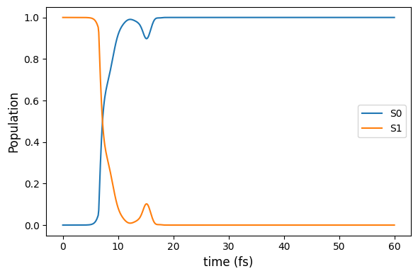
The information in the resulting dataframe can be easily plotted using the seaborn or matplotlib libraries. In the example, the S0 and S1 populations are plotted over time for one specific trajectory using matplotlib.
[16]:
# Selects the data associated to TRAJ1.
df_TRAJ1 = df_pop[df_pop['TRAJ'] == 1 ]
[17]:
# First, some code lines to set up the plot.
import matplotlib.pyplot as plt
fig , ax = plt.subplots(figsize=(6,4))

# Then, giving labels to the axis...
ax.set_ylabel('Population', fontsize=12)
ax.set_xlabel('time (fs)'      , fontsize=12)

# ... and informing the what should be plotted. x-axis is time and y-axis is the respective populations.
plt.plot(df_TRAJ1['time'], df_TRAJ1['Pop1'], label='S0')
plt.plot(df_TRAJ1['time'], df_TRAJ1['Pop2'], label='S1')

# And, finally, setting up the data labels.
ax.legend(loc='best', frameon=None)
plt.tight_layout()
plt.show()
4. nac_norm()
Calculate the norm of the nonadiabatic coupling matrices for each pair of states. After running this function, the properties dataset sored in the class variable GetProperties.dataset will be updated with the computed NACs norm data. Before running this function, let’s first take a look at the current state of the properties dataset.
[18]:
properties.dataset
[18]:
| TRAJ | time | State | Total_Energy | Hops_S12 | S1 | Hops_S21 | DE21 | Root2 | only_root2 | only_root1 | f_21 | Pop1 | Pop2 | |
|---|---|---|---|---|---|---|---|---|---|---|---|---|---|---|
| 0 | 1 | 0.0 | 2 | -6271.713990 | 0 | -6276.740507 | 0 | 3.852182 | -6267.861809 | -6267.861809 | NaN | -0.004430 | 0.000000 | 1.000000e+00 |
| 1 | 1 | 0.1 | 2 | -6271.714018 | 0 | -6276.777841 | 0 | 3.839637 | -6267.874380 | -6267.874380 | NaN | -0.004396 | 0.000001 | 9.999989e-01 |
| 2 | 1 | 0.2 | 2 | -6271.714045 | 0 | -6276.812753 | 0 | 3.825025 | -6267.889020 | -6267.889020 | NaN | -0.004357 | 0.000004 | 9.999964e-01 |
| 3 | 1 | 0.3 | 2 | -6271.714072 | 0 | -6276.844754 | 0 | 3.808371 | -6267.905701 | -6267.905701 | NaN | -0.004313 | 0.000006 | 9.999936e-01 |
| 4 | 1 | 0.4 | 2 | -6271.714099 | 0 | -6276.873408 | 0 | 3.789650 | -6267.924449 | -6267.924449 | NaN | -0.004266 | 0.000008 | 9.999916e-01 |
| ... | ... | ... | ... | ... | ... | ... | ... | ... | ... | ... | ... | ... | ... | ... |
| 2979 | 5 | 59.6 | 1 | -6271.412760 | 0 | -6274.238936 | 0 | 5.447232 | -6265.965528 | NaN | -6274.238936 | -0.006061 | 1.000000 | 3.998308e-07 |
| 2980 | 5 | 59.7 | 1 | -6271.412760 | 0 | -6274.225956 | 0 | 5.497873 | -6265.914888 | NaN | -6274.225956 | -0.006146 | 1.000000 | 3.824953e-07 |
| 2981 | 5 | 59.8 | 1 | -6271.412760 | 0 | -6274.214527 | 0 | 5.548187 | -6265.864574 | NaN | -6274.214527 | -0.006231 | 1.000000 | 3.651934e-07 |
| 2982 | 5 | 59.9 | 1 | -6271.412733 | 0 | -6274.204813 | 0 | 5.598147 | -6265.814586 | NaN | -6274.204813 | -0.006318 | 1.000000 | 3.479378e-07 |
| 2983 | 5 | 60.0 | 1 | -6271.412733 | 0 | -6274.196922 | 0 | 5.647644 | -6265.765089 | NaN | -6274.196922 | -0.006405 | 1.000000 | 3.307478e-07 |
2984 rows × 14 columns
[19]:
df_with_nacs = properties.nac_norm()
Reading nonadiabatic couplings from TRAJ1...
Reading nonadiabatic couplings from TRAJ2...
Reading nonadiabatic couplings from TRAJ3...
Reading nonadiabatic couplings from TRAJ4...
Reading nonadiabatic couplings from TRAJ5...
[20]:
# Updated properties dataset
properties.dataset
[20]:
| TRAJ | time | State | Total_Energy | Hops_S12 | S1 | Hops_S21 | DE21 | Root2 | only_root2 | only_root1 | f_21 | Pop1 | Pop2 | NAC_S2S1 | |
|---|---|---|---|---|---|---|---|---|---|---|---|---|---|---|---|
| 0 | 1 | 0.0 | 2 | -6271.713990 | 0 | -6276.740507 | 0 | 3.852182 | -6267.861809 | -6267.861809 | NaN | -0.004430 | 0.000000 | 1.000000e+00 | 0.715162 |
| 1 | 1 | 0.1 | 2 | -6271.714018 | 0 | -6276.777841 | 0 | 3.839637 | -6267.874380 | -6267.874380 | NaN | -0.004396 | 0.000001 | 9.999989e-01 | 0.714953 |
| 2 | 1 | 0.2 | 2 | -6271.714045 | 0 | -6276.812753 | 0 | 3.825025 | -6267.889020 | -6267.889020 | NaN | -0.004357 | 0.000004 | 9.999964e-01 | 0.715183 |
| 3 | 1 | 0.3 | 2 | -6271.714072 | 0 | -6276.844754 | 0 | 3.808371 | -6267.905701 | -6267.905701 | NaN | -0.004313 | 0.000006 | 9.999936e-01 | 0.715848 |
| 4 | 1 | 0.4 | 2 | -6271.714099 | 0 | -6276.873408 | 0 | 3.789650 | -6267.924449 | -6267.924449 | NaN | -0.004266 | 0.000008 | 9.999916e-01 | 0.716958 |
| ... | ... | ... | ... | ... | ... | ... | ... | ... | ... | ... | ... | ... | ... | ... | ... |
| 2979 | 5 | 59.6 | 1 | -6271.412760 | 0 | -6274.238936 | 0 | 5.447232 | -6265.965528 | NaN | -6274.238936 | -0.006061 | 1.000000 | 3.998308e-07 | 0.368913 |
| 2980 | 5 | 59.7 | 1 | -6271.412760 | 0 | -6274.225956 | 0 | 5.497873 | -6265.914888 | NaN | -6274.225956 | -0.006146 | 1.000000 | 3.824953e-07 | 0.363998 |
| 2981 | 5 | 59.8 | 1 | -6271.412760 | 0 | -6274.214527 | 0 | 5.548187 | -6265.864574 | NaN | -6274.214527 | -0.006231 | 1.000000 | 3.651934e-07 | 0.359262 |
| 2982 | 5 | 59.9 | 1 | -6271.412733 | 0 | -6274.204813 | 0 | 5.598147 | -6265.814586 | NaN | -6274.204813 | -0.006318 | 1.000000 | 3.479378e-07 | 0.354702 |
| 2983 | 5 | 60.0 | 1 | -6271.412733 | 0 | -6274.196922 | 0 | 5.647644 | -6265.765089 | NaN | -6274.196922 | -0.006405 | 1.000000 | 3.307478e-07 | 0.350316 |
2984 rows × 15 columns